How To Use qzwslrm

library(qzwslrm)

Installation

The package qzwslrm can be installed from Github

# if (!is.element("devtools", installed.packages()) install.packages("devtools")
devtools::install_github("fbzwsqualitasag/qzwslrm")

Disclaimer

This is a short introduction on how to use the package qzwslrm.

Abstract

The package qzwslrm implements the computation of the EBV validation statistics using the LR-method. This requires two vectors with EBV for the same group of animals. One vector contains EBV for the group of animals estimated using the full dataset (‘whole’) and the second vector contains EBV for the same group of animals estimated using only a partial dataset (‘partial’).

Given two vectors vec_ebv_whole and vec_ebv_partial with EBV for the same group of animals from whole data and partial data, respectively, the following command computes a first set of validation statistics.

l_val_result <- val_ebv_lrm(pvec_ebv_partial = tbl_solani_partial$ebv, 
                            pvec_ebv_whole = tbl_solani_whole$ebv)

Usage

As shown above, the function val_ebv_lrm() is the central function that computes the validation statistics. The function val_ebv_lrm() returns a list with all validation statistics. The results can be shown using the summary function summary_lrm() or by converting them into a tibble.

Results

The function summary_lrm() can be used to show a summary of the validation statistics

summary_lrm(l_val_result)
#> 
#> Bias between partial and whole:  -0.0061
#> Regression whole on partial:         1.0377
#> Correlation whole and partial:       0.9873
#> Regression partial on whole:         0.9393

If the results should be displayed as a table this can be done by converting it to a tibble and using then the function knitr::kable().

tbl_lrm <- tibble_lrm(l_val_result)
knitr::kable(tbl_lrm)

Validation Statistic	Value
Bias between partial and whole	-0.0061
Regression whole on partial	1.0377
Correlation whole and partial	0.9873
Regression partial on whole	0.9393

Scatterplot

The comparison of the two vectors of EBV can also be illustrated by a scatterplot. Such a plot can be generated using the function scatterplot_lrm().

tbl_ebv_whole <- readr_ebv(ps_path = qzwslrm_example_solani("whole"), ps_format = "table",
                            pn_ebv_col_idx = 4)
tbl_ebv_partial <- readr_ebv(ps_path = qzwslrm_example_solani("partial"), ps_format = "table",
                              pn_ebv_col_idx = 4)
p <- scatterplot_lrm(tbl_ebv_whole, tbl_ebv_partial)
print(p)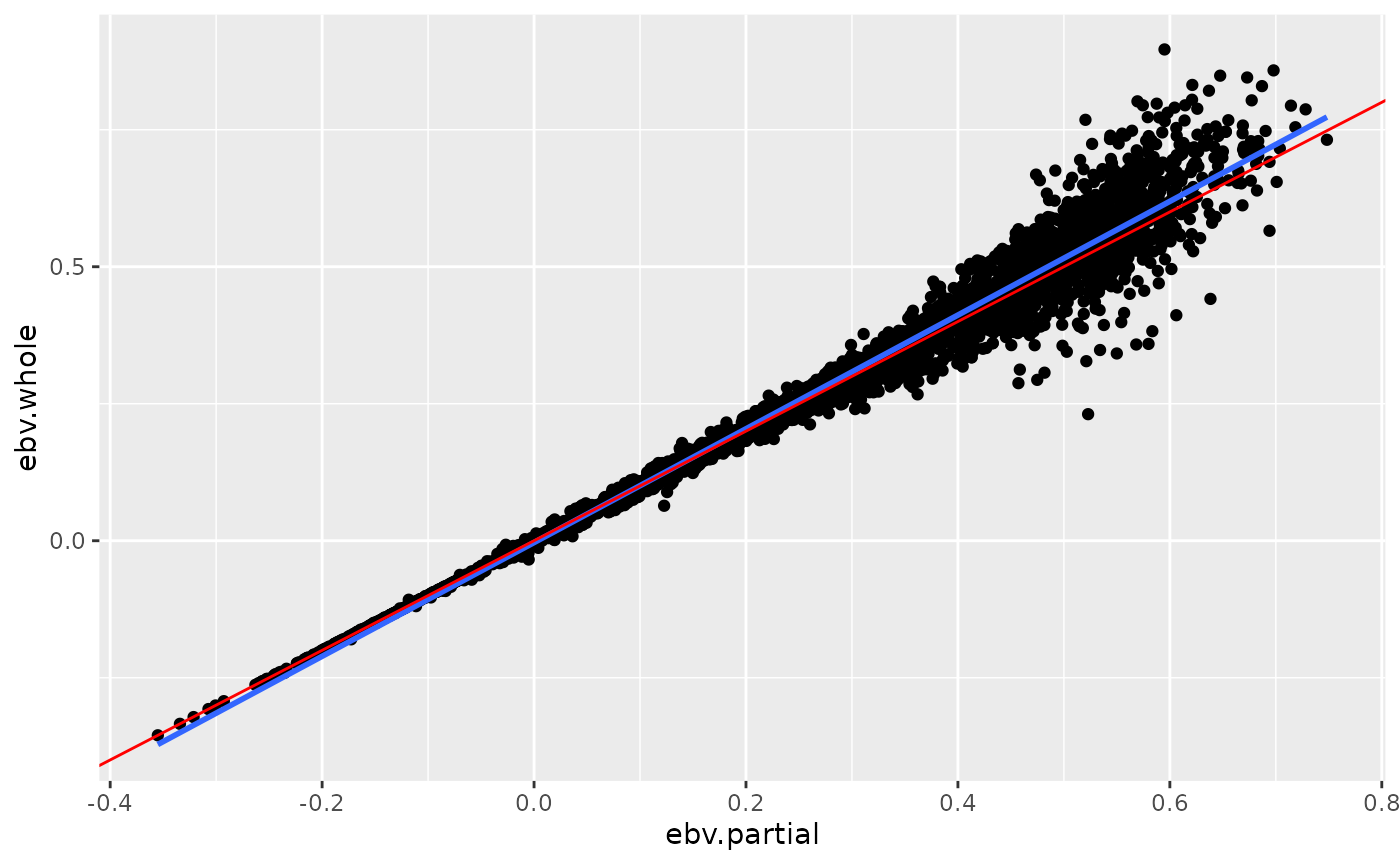

The above plot shows for each animal the pair of EBV from the whole and from the partial dataset. The blue line corresponds to the linear smoother which is drawn based on the points. The red line corresponds to the line with a slope equal to one which is the expected regression line for the ‘whole’ on the ‘partial’ EBV.

The function scatterplot_lrm() requires as input two dataframes with two columns. The first column contains the animal ID and the second column contains the EBV.